Working with Spreadsheets
Related Documentation
- Overview of Spreadsheet Studies
- Using Spreadsheet Studies
- Spreadsheet Systems, Alerts and Automated Trading
- Spreadsheet Study Inputs
- Referencing Other Charts in Spreadsheet Study Formulas
- Spreadsheet Studies Special Tasks
- Sharing Your Spreadsheet Study With Another User
- Working with Spreadsheets
- Spreadsheet Functions
- Spreadsheet Example Formulas and Usage
On This Page
- Introduction
- Difference Between New and Old Spreadsheets
- Difference Between Sheets and Spreadsheets
- Spreadsheet Menu Commands
- Creating and Opening Spreadsheets
- Spreadsheet Cells
- Activating and Viewing (Selecting) Sheets within a Spreadsheet
- Entering Data
- Filling Cells
- Undo
- Formulas
- Viewing Formula Expression Tree
- Operators
- User Defined Names
- True and False Values
- Decimal and Function Delimiters
- Cell and Range Selection
- Cell Formatting
- Color Settings
- Cell and Range References
- Inserting and Deleting Rows and Columns
- Keyboard Commands
- Spreadsheet Error Codes
- Rename a Sheet
- Floating-Point Values and Comparisons When Using the Spreadsheet Study
- Accessing a Backup Spreadsheet File
- Saving a Sheet in Text Format
- Different Methods to Get Data Into and Out of Spreadsheets
Introduction
Sierra Chart has very advanced built-in Spreadsheets. Sierra Chart spreadsheets are Excel compatible in the sense that they use the same formula format and support most of the same functions.
Spreadsheets are used to create custom Studies, Trading Systems and advanced Alerts by using one of the available Spreadsheet Studies.
Spreadsheets can also be used to contain detailed continuously updating quotes for a powerful Quote Board. For more information on continuously updating quotes, refer to the Getting Quotes documentation page.
Difference Between New and Old Spreadsheets
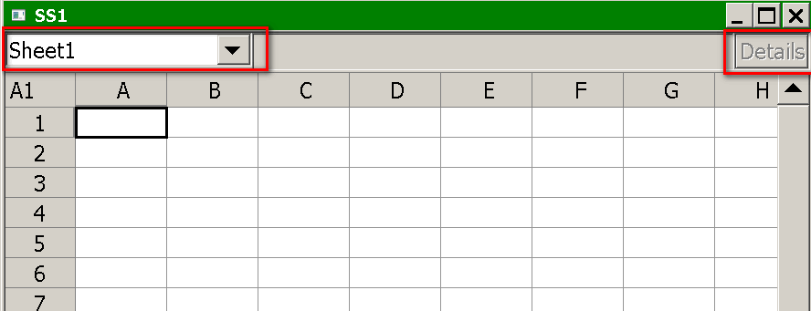
Newer versions of Sierra Chart use what are called New Spreadsheets and replace the previous Old Spreadsheets in older versions. New Spreadsheets is a completely new Spreadsheet component developed by Sierra Chart. You can tell if you are using New Spreadsheets by the appearance of the Spreadsheet by looking at the top of the Spreadsheet window. Here is an example:
The top of the Window >> Message Log also will indicate whether you are using New Spreadsheets or Old Spreadsheets. At the present time almost all users are using New Spreadsheets.
All of the Spreadsheet documentation on this website applies to New Spreadsheets only.
The following are the limitations, advantages and differences when using New Spreadsheets compared with Old Spreadsheets:
-
New Spreadsheets do not support all of the functions that are available in Old Spreadsheets. For example functions that are not relevant like loan related functions are not supported. All of the most relevant core and basic Spreadsheet functions are supported. The following functions are not supported: COUNTIF, AVERAGEIF, MAXIF, MINIF, SUMIF. For an alternative to these functions, refer to Using the Equivalent of COUNTIF, AVERAGEIF, MAXIF, MINIF, SUMIF. For a list of the Spreadsheet functions supported in New Spreadsheets, refer to Spreadsheet Functions.
-
New Spreadsheets do not support the user interface which is known as Range Explorer and Workbook Explorer.
-
New Spreadsheets do not support referencing data across Spreadsheets by specifying the name of the Spreadsheet in a cell reference. It is only possible to make references to other Sheets within the same Spreadsheet. There are ways of designing your use of Spreadsheets, so this is not required. Refer to this discussion thread for alternatives. The main solution is to use the Chart Data Output Sheet Number Spreadsheet Study Input to control what Sheet within the Spreadsheet the data is outputted to and is used by the Spreadsheet study.
-
New Spreadsheets have multiple window views into the same Spreadsheet Sheet. This is accessed through Spreadsheet >> New View.
-
In New Spreadsheets, when Sheets are added or removed, existing sheets still maintain their reference to the same chart when using the Spreadsheet study.
-
New Spreadsheets have a new referencing method for chart data and studies which automatically adjust to studies being reordered. This prevents having to change formulas when studies are inserted or reordered.
-
Refer to this video demonstrating how to enter data and formulas with New Spreadsheets.
-
The Spreadsheet Studies for New Spreadsheets support outputting Volume at Price data. All of the Spreadsheet studies have an Output Volume at Price Data study input which can be set to Yes. When this is set to Yes, the Volume at Price data will be outputted beginning at column BA.
-
The limitations which exist in New Spreadsheets, exist because of the very high degree of complexity to implement them and to support them. Spreadsheets are complicated enough without adding unnecessary complexity. We have a responsibility to ensure the Spreadsheets are fast, are reliable and can be properly maintained and supported. So these limitations are likely to always be limitations but they really are not limitations because the core spreadsheet functionality is provided and it executes very fast and accurately.
Difference Between Sheets and Spreadsheets
A spreadsheet window contains one or more Sheets. Each of these Sheets is a Spreadsheet itself and can refer to other Sheets within the overall Spreadsheet window.
A Spreadsheet is a single window in Sierra Chart that can be saved to a file and opened. They are separate from Chartbooks which are collections of chart windows.
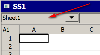
The individual Sheets in a Spreadsheet can be selected from the drop-down list menu at the top left of the Spreadsheet window. Refer to the image below.
Using Keyboard to Access Sheets
When the list box of Sheets at the top left has the focus, you can use the Up and Down arrow keys on your keyboard to cycle through the Sheets. When each Sheet is selected in the list, it will immediately become active. This allows you to quickly cycle through the Sheets to view each one with the up and down arrow keys.
Spreadsheet Menu Commands
The Sierra Chart menus contains commands for Spreadsheets. Documentation for these menu commands can be found on the File Menu and Spreadsheet Menu documentation pages.
Creating and Opening Spreadsheets
To create a new Spreadsheet, select File >> New Spreadsheet on the menu.
To open an existing Spreadsheet: Select File >> Open Spreadsheet on the menu. The Open Spreadsheet window will display. Select a Spreadsheet file in the list. Press the Open button.
The File Type drop down list box in the Open Spreadsheet window lists the different types of Spreadsheet files you can open. Select the type of file you want to open from the list if you want to open a type other than the default. For example, you can open a text file where the values are separated by a comma or tab character.
New and existing Spreadsheet windows for Spreadsheet Studies applied to a chart, are automatically created or opened by the Spreadsheet Study, Spreadsheet System/Alert and Spreadsheet System for Trading studies.
When opening a Chartbook that contains charts that use one of the Spreadsheet Studies, the very first Spreadsheet Study that is opening the Spreadsheet file will set the active Sheet to the Sheet it is outputting data to. Any other Spreadsheet Studies which reference the same Spreadsheet file, will not change the active Sheet in that Spreadsheet window.
Spreadsheet Cells
Spreadsheets contain rows and columns of cells. Spreadsheet cells can contain formulas, numbers, dates, times, text, logical values (TRUE, FALSE), or error values.
The active cell is the one where the Spreadsheet highlight box is located.
Activating and Viewing (Selecting) Sheets within a Spreadsheet
A Sierra Chart Spreadsheet window contains one or more Sheets. At the top left of the Spreadsheet window, there is a list box which contains all of the Sheets within the Spreadsheet window. Select the particular Sheet you want to display from that list.
If the Spreadsheet is already visible, then it can be made active, if it is not already, by left clicking with your Pointer anywhere on the Spreadsheet window.
Entering Data
To select a cell, first activate the Spreadsheet if it is not already active, by left clicking anywhere on it with your Pointer.
Use the keyboard arrow keys to move to a cell or select a cell by pointing to it with your Pointer and left click it with your Pointer.
To enter data on a cell in a Spreadsheet in the version of Sierra Chart with New Spreadsheets, you first need to left click 2 times with your Pointer in the cell to open the edit box for the cell. Enter the data. Press the OK button to save it into the cell. Refer to the image below.
Unlike when entering data into Formulas and Functions, dates, times, and text should not be enclosed quotation marks when entered directly into cells.
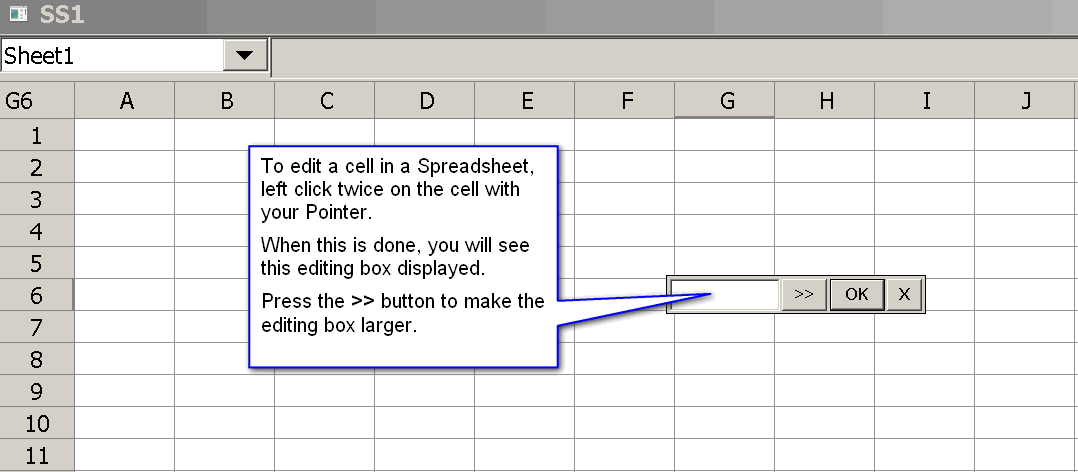
To expand the cell editing window, press the >> button. You can invoke this button, through the keyboard. Press TAB followed by SPACE. In the compact edit window, the focus is by default on the edit control. By pressing TAB, that moves the focus to the expand (>>) button. And by pressing SPACE when the focus is on the expand button will click that button and expand the edit window.
Filling Cells with Value or Formula
If you have a value or formula in a cell and you want to fill other cells with this same data, then perform the following steps:
- Select the cell or cells that you wish to copy from. Copy the values or formulas by selecting Spreadsheet >> Copy Value or Spreadsheet >> Copy Formula respectively.
- Select the range of cells that you want to be filled in with the contents of the originally selected cell or cells.
- Perform a paste operation by selecting Spreadsheet >> Paste. If you are copying a formula, then the cell references will be automatically adjusted unless they are absolute references.
- It is also possible to use the Spreadsheet >> Copy Down and Spreadsheet >> Copy Right commands to fill cells.
Undo
Selecting Spreadsheet >> Undo will reverse the last performed action on the spreadsheet. It will only undo one single action, it does not store multiple actions to undo.
If the last edit was performed on a different sheet than the one that is currently displayed, the system will display the sheet with the last edit and perform the undo action.
The following are the only items that can be undone. Anything not listed here is not available through the Undo function.
- Edits made in a cell
- Edits made to a cell's comment
- Edits made to both a cell and its comment through the expanded edit window
- The last Undo action (a Redo action)
Formulas
Formulas can be entered into Spreadsheet cells to perform calculations on data.
A formula starts with an equals sign (=) and can contain Spreadsheet Functions, numbers, Named Constants, cell references, text strings (text needs to be in quotation marks), logical values (TRUE, FALSE), and Operators.
Most formulas that can be used in Excel can be used in Sierra Chart Spreadsheets.
When entering numbers and formulas, keep in mind to use the proper delimiters in your numbers and formulas, according to your Region Setting. For more information, see the Decimal and Function Delimiters section.
Examples:
= A2 + 10 — If A2 has the value 5, then this formula returns 15.
= SUM( B2:B10 ) — This formula uses the SUM function. The sum of cells B2 through B10 is returned.
= C10 — Returns the value in cell C10.
Dates and/or Times when entered into cells are stored as Serial DateTime Values, which are numeric values. Arithmetic can be used on these numeric values.
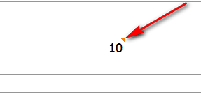
When a Sheet cell contains a formula, at the top right of the cell there is a red indicator indicating this. Refer to the image below.
Viewing Formula Expression Tree
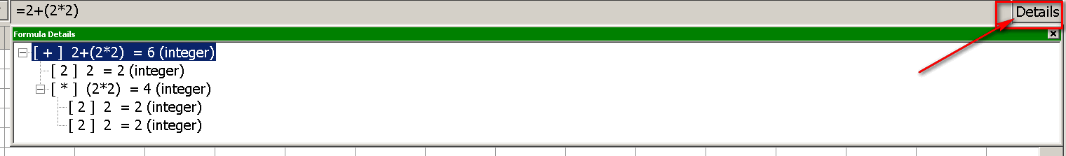
It is supported to see the formula expression tree for a selected formula. The formula expression tree displays the result of each subexpression. This is very useful to debug a formula that is giving an error.
This feature is accessed by selecting a cell and then pressing the Details button at the top right of the Spreadsheet. Refer to image below.
Double-clicking or pressing the Enter/Return key on an item in the formula expression tree list that is either a reference or returns a reference will immediately jump to the referenced cell.
When using the AND function, the formula expression tree may show (not evaluated) for one or more of the expressions. This is normal and is due to the underlying need of the AND function to have all expressions be true in order for the AND function to be true. Therefore, if the first expression returns false, no further processing is required and additional expressions are not evaluated.
Operators
Unary Operators
Unary Negation (-)
Example: = - A1
The result of this operator is the negative of the value of the given operand. For example, if the value is 2, the result will be -2; if the value is -2, the result will be 2. This operator only works on numeric value types.
Unary Logical Inversion (Not) (!)
Example: = ! A1
The result of this operator is the logical inverse of the value of the given operand. If the value is TRUE, the result will be FALSE; if the value is FALSE, the result will be TRUE. This operator only works on logical (boolean) value types.
If the value type of the operand is not compatible with the operator, such as trying to negate a string, or trying to 'not' a number, the operation will result in a #VALUE! error.
If the value of the operand is an error value, that error value will be passed through as the result of the operation.
If the operand has no value, then the result of the operation will also be no value.
Arithmetic Operators
Addition (+)
Example: = A1 + B1
The result of this operator is the value of the second operand (B1) added to the value of the first operand (A1). This works with text values by concatenating the values together. This operator also behaves as an OR operator for logical (boolean) values.
Subtraction (-)
Example: = A1 - B1
The result of this operator is the value of the second operand (B1) subtracted from the value of the first operand (A1). This operator also behaves as an XOR operator for logical (boolean) values.
Multiplication (*)
Example: = A1 * B1
The result of this operator is the value of the first operand (A1) multiplied by the value of the second operand (B1). This operator also behaves as an AND operator for logical (boolean) values.
Division (/)
Example: = A1 / B1
The result of this operator is the value of the first operand (A1) divided by the value of the second operand (B1). If the value of the second operand is 0, the result is a #DIV/0! error.
Exponentiation (^)
Example: = A1 ^ B1
The result of this operator is the value of the first operand (A1) raised to the power of the value of the second operand (B1). 0^0 will give a result of 1. 0 raised to a negative number will result in a #DIV/0! error, because it is equivalent to dividing by zero. A negative number raised to a number that is not whole will result in a #NUM! error, because imaginary numbers are not supported. This operator also behaves as an AND operator for logical (boolean) values.
If the types of the values of the operands are not compatible with the operator, such as trying to divide logical (boolean) values, or if the types of the values are not compatible with each other, such as trying to add a number to a text value, the operation will result in a #VALUE! error.
If the value of either operand is an error value, that error value will be passed through as the result of the operation. If both operands are errors, the error value from the first operand will be passed through as the result.
If both operands are non-values (referencing an empty cell), the result of the operation will also be an empty value (no value).
Comparison Operators
Less (<)
Example: = A1 < B1
The result of this operator will be TRUE if and only if the value of the first operand (A1) is less than the value of the second operand (B1). If the first value is not less than the second value, the result will be FALSE.
Less or Equal (<=)
Example: = A1 <= B1
The result of this operator will be TRUE if and only if the value of the first operand (A1) is either less than or equal to the value of the second operand (B1). If the first value is not less than or equal to the second value, the result will be FALSE.
Equal (=)
Example: = A1 = B1
The result of this operator will be TRUE if and only if the value of the first operand (A1) is equal to the value of the second operand (B1). If the first value is not equal to the second value, the result will be FALSE. Unlike most operators, if either operand is an error value, these values will be compared the same as any other value type.
Greater or Equal (>=)
Example: =A1 >= B1
The result of this operator will be TRUE if and only if the value of the first operand (A1) is either greater than or equal to the value of the second operand (B1). If the first value is not greater than or equal to the second value, the result will be FALSE.
Greater (>)
Example: = A1 > B1
The result of this operator will be TRUE if and only if the value of the first operand (A1) is greater than the value of the second operand (B1). If the first value is not greater than second value, the result will be FALSE.
Not Equal (<>)
Example: = A1 <> B1
The result of this operator will be TRUE if and only if the value of the first operand (A1) is not equal to the value of the second operand (B1). If this is not the case, the result will be FALSE. Unlike most operators, if either operand is an error value, these values will be compared the same as any other value type.
If neither operand has a value (references an empty cell), the operands are considered equal.
If the types of the values of the operands are not compatible with each other, such as trying to compare a number to a text value, the operation will result in a #VALUE! error.
Aside from the equal (=) and not equal (<>) operators, if the value of either operand is an error value, that error value will be passed through as the result of the operation. If both operands are errors, the error value from the first operand will be passed through as the result.
Chained Operators
Multiple comparison operators that share operands can be chained together. For example, the formula = A1 = B1 = 0 will return TRUE if and only if the values of both A1 and B1 are equal to 0. This gives the same result as the formula = AND( A1 = 0, B1 = 0 ). Another example is the formula = A1 < A2 < A3 < A4, which returns true if and only if the values of A1 through A4 are ascending and not equal. This gives the same result as the formula = AND( A1 < A2, A2 < A3, A3 < A4 ).
Use parentheses, ( ), around expressions to change order of precedence.
User Defined Names
The new spreadsheets do not support custom names defined by the user. However, various predefined names can be used within spreadsheet formulas.
Named Constants
The following names are already defined and set to the values listed.
Months
| Name | Value |
|---|---|
| JANUARY | 1 |
| FEBRUARY | 2 |
| MARCH | 3 |
| APRIL | 4 |
| MAY | 5 |
| JUNE | 6 |
| JULY | 7 |
| AUGUST | 8 |
| SEPTEMBER | 9 |
| OCTOBER | 10 |
| NOVEMBER | 11 |
| DECEMBER | 12 |
These are useful with the DATE function. For example: = DATE( 2001, JANUARY, 1 ) results in the date value for January 1st, 2001.
Days of the Week
| Name | Value |
|---|---|
| SUNDAY | 1 |
| MONDAY | 2 |
| TUESDAY | 3 |
| WEDNESDAY | 4 |
| THURSDAY | 5 |
| FRIDAY | 6 |
| SATURDAY | 7 |
These are useful with the WEEKDAY function. For example: = WEEKDAY( A1 ) = FRIDAY results in TRUE if the date value in cell A1 is a Friday.
Math Constants
| Name | Value |
|---|---|
| E | 2.71828182845904523536 |
| PI | 3.14159265358979323846 |
These are useful with the various mathematics related functions. For example: = LN( E ) results in 1.0.
True and False Values
In Sierra Chart Spreadsheets, True is represented by 1 and False is represented by 0. So a formula that returns TRUE will display 1 in a cell and a formula that returns FALSE will display 0.
It is possible to format a cell to display TRUE when it contains 1.0 and FALSE when it contains 0.0. This can be done by selecting the cell or a range of cells and selecting Spreadsheet >> Number Format and choosing the TRUE/FALSE Number Format.
Decimal and Function Delimiters
The delimiters for decimal numbers and function parameters can be changed to suit different region preferences. Two options are available:
- Use full stop (.) decimal delimiter, and comma (,) function delimiter.
- Use comma (,) decimal delimiter, and semicolon (;) function delimiter.
This setting for decimal and function delimiters is found in the Spreadsheet Settings window, which can be accessed from the menu item Global Settings >> Spreadsheet Settings.
The decimal delimiter is the character that is used for the decimal point in decimal numbers. A number using a full stop (.) decimal delimiter would look like 1.25, while the same number using a comma (,) decimal delimiter would look like 1,25.
The function parameter delimiter is the character that is used to separate parameters in formula functions. An example of the SUM function using a comma (,) parameter delimiter would look like =SUM( A1, B2, C3 ), while the same function using a semicolon (;) parameter delimiter would look like =SUM( A1; B2; C3 ).
Cell and Range Selection
Click and hold your left Pointer button and drag through a range of cells to select them. Or press the SHIFT key and use the keyboard navigation keys to select a range of cells.
A single cell is also considered a range or a selection. It is range or selection of just one cell.
To select an entire column or row, left click with your Pointer the column or row header of a Sheet. Headers are along the top and left of the Spreadsheet. If you left click and drag with your Pointer across the headers you can select multiple columns or rows.
The active cell has a thick border around it. Other selected cells are shaded.
Cell Formatting
Each cell can be individually set to display numeric values using a specific value format, as well as using specific text and background colors.
The value format for the currently selected cell or range of cells can be set through the menu item Spreadsheet >> Number Format.
Likewise, the text and background colors for the currently selected cell or range of cells can be set through the menu item Spreadsheet >> Cell Properties.
The font, font style, and font size used for the text in cells cannot be changed for individual cells, but can be set for all spreadsheets through the menu item Spreadsheet >> Change Font.
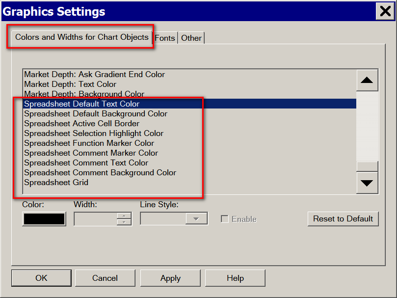
Color Settings
There are various color settings available for Spreadsheets. They are set through Global Settings >> Graphics Settings >> Colors and Widths. Refer to the image below.
Cell and Range References
General
A reference refers to the contents of a cell or a range of cells. References are used in formulas. The reference specifies a cell by referring to the row and column position of the cell. The reference uses the row and column headings in the Spreadsheet. Example: A1 refers to the cell at column A and row 1. To reference a range of cells, use a colon (:) between the cell reference at the top left of the range and the cell reference at the bottom right of the range.
Basic Reference Examples:
B1 refers to cell at column B and row 1.
A1:B4 refers to the range that includes all cells in columns A and B of rows 1, 2, 3, and 4.
A1:A10 refers to the range that includes all cells in column A of rows 1 to 10.
Relative and Absolute References
There are relative and absolute cell references. Relative references refer to a cell using offsets that the cell being referenced is to the cell that contains the reference.
When a cell containing a Relative reference is copied, the reference is adjusted to refer to a new cells with the same offsets that the original cell had to the cells it was referencing.
Absolute references refer to a cell at an exact location. When a cell containing an Absolute reference is copied, the reference will not change. Absolute references are specified with a dollar sign ($) in front of the row and/or column that is to be absolute.
References can be part absolute and part relative.
Relative and Absolute Reference Examples:
B1 Relative reference to cell B1. It if is in cell A1 and copied to A2, then it will refer to B2 since the reference refers to one cell to the right in the same row.
$C$4 Absolute reference cell C4.
$D1 Absolute column reference and relative row reference to cell D1.
A$2 Relative column reference and absolute row reference to cell A2.
ID1.SG1@$3Relative column reference and absolute row reference to Study Subgraph. For additional information, refer to References to Study Subgraph Columns when using the Spreadsheet Study
References to Other Sheets within a Spreadsheet
Sierra Chart Spreadsheets support references to cells in other Sheets within the same Spreadsheet window. To reference cells in a particular Sheet in the same Spreadsheet, use the following format. Remember that references are used in formulas, and formulas begin with an equals sign (=).
Format: 'SheetName'!CellReference
If the Sheet Name does not contain any spaces the single quotes can be omitted.
Examples:
= Sheet1!A1
='First Sheet'!A1
References to Other Spreadsheets Windows
References between Sheets among different Spreadsheet windows is not supported. A Spreadsheet window is a separate distinct window opened through File >> Open Spreadsheet or automatically opened by a Spreadsheet Study.
However, follow the instructions below to use multiple Spreadsheet studies which output to the same named Spreadsheet and supports sharing/referencing of data between the Sheets within the Spreadsheet window/collection.
- For each chart that you want to have chart data and study data outputted to a Sheet in a Spreadsheet, add one of the Spreadsheet Studies to the chart.
- For each instance of the Spreadsheet study being used, make sure the Spreadsheet Name setting in the Study Settings window set to the same name.
- Make sure that each chart is outputting data to a different Sheet within the same Spreadsheet. This is done through the Chart Data Output Sheet Number or Chart Data Open Sheet Name Inputs. Normally this will be the case. However, if you are using the same named Spreadsheet among different Chartbooks, then you have to be careful about this and make sure that each chart is outputted to a different Sheet.
- Now that the chart data and study data is being outputted to the different Sheets within the same Spreadsheet, you can then use cell references to reference the data between the Sheets.
- If there are two Sheets you want to be able to view at the same time in the same Spreadsheet window, this is accomplished by going to the Spreadsheet window and selecting Spreadsheet >> New View. This other view can be set to display a different Sheet.
You also have the ability through Window >> Detach/Attach Window to detach it from the main Sierra Chart window.
References to Study Subgraph Columns when using the Spreadsheet Study
It is supported to reference Study Subgraph columns when using the Spreadsheet Study using a format which constantly refers to a specific Study Subgraph on the chart even if studies are reordered on the Spreadsheet Sheet, or if other studies that are not being referenced are no longer being outputted to the Spreadsheet Sheet.
This referencing method is also valid when referencing the chart bar data from the main price graph which is outputted to columns A through G on the Sheet.
The cell reference format is [Study ID].[Subgraph number]@[Row number].
The Study ID number is displayed after the study in the Analysis >> Studies >> Studies to Graph list. The Subgraph number (SG#) is displayed on the Subgraphs tab of the Study Settings window after each Subgraph name.
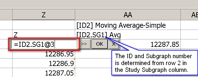
The Study ID and Subgraph number which are separated by a period are displayed at row 2 in the Study Subgraph or main price graph Column on the Sheet in the Spreadsheet window. Refer to the image below.
Example: ID1.SG1@3.
For example, in the image below instead of using AA3 to reference the value of the Moving Average Subgraph at row 3, the new direct Study Subgraph reference method is used instead.
Example to create range when using direct Study Subgraph cell references: =SUM(ID1.SG1@3:ID1.SG1@100).
Related to this, it is also supported to update Sheet cell references when inserting and deleting rows and columns. Refer to Inserting and Deleting Rows and Columns. The setting is Global Settings >> Spreadsheet Settings >> Reference Modification When Inserting and Deleting Rows or Columns.
Programmatically Creating Study Subgraph Columns References
These study subgraph column references can be used with the INDEX and OFFSET formula functions to access specific cells or ranges of cells within those columns.
For example, the first cell in the column can be accessed using either INDEX(ID1.SG1:ID1.SG1, 3) or OFFSET(ID1.SG1@3, 0, 0). Both of these are still equivalent to ID1.SG1@3, but more advanced formulas—including references to other cell values—can be used with these formula functions.
For example, the Number of Rows value in cell J30 can be used to get the last value in the column using either INDEX(ID1.SG1:ID1.SG1, 3 + $J$30 - 1) or OFFSET(ID1.SG1@3, $J$30 - 1, 0).
The OFFSET formula function can additionally be used to get ranges of values, such as OFFSET(ID1.SG1@3, 0, 0, 10, 1) will return a range of the top 10 rows in the column.
The INDEX formula function can be used to get individual cells within a range of columns, such as INDEX(ID1.SG1:ID1.SG3, 3, 2) to get the first value (in row 3) in the 2nd column.
Inserting and Deleting Rows and Columns
To insert or delete rows or columns within a Sheet, refer to the documentation for the following Spreadsheet menu commands:
- Spreadsheet >> Insert Row
- Spreadsheet >> Insert Column
- Spreadsheet >> Delete Row
- Spreadsheet >> Delete Column
References within existing formulas can be updated when inserting or deleting rows or columns. The setting that controls this is Global Settings >> Spreadsheet Settings >> Reference Modification When Inserting and Deleting Rows or Columns.
The documentation for this setting is as follows:
Do Not Update References
References in formulas will continue referencing the same literal cell address, even if the referenced cell was moved or deleted as a result of the insert or delete operation.
Example
A1:=A3
The following is the result of an operation to insert a row at row 2.
A1:=A3
Update References To Match Moved Cells
References in formulas will be updated so that they refer to the new location of cells that were moved as a result of the insert or delete operations. If a referenced cell is deleted, the referenced will change to a #REF! error.
Example
A1:=A3
The following is the result of an operation to insert a row at row 2.
A1:=A4
Keyboard Commands
Arrow Keys
The Up, Down, Left, and Right arrow keys move the active cell selection one cell up, down, left, and right.
Holding down the Ctrl key while using the arrow keys will cause the active cell selection to skip to the edge of a block of cells. If the current active cell selection is within a block of non-empty cells, the active cell selection will jump to the edge of the block. If the current active cell selection is already on the edge of a block, where the next cell is empty, or on an empty cell, the active cell selection will jump to the next non-empty cell.
Home/End
The Home key moves the active cell selection to the first column of the active row, and the End key moves it to the last non-empty cell in the active row.
If the Ctrl key is held down, the Home and End keys instead move to the first and last cells of the current active column.
Page Up/Page Down
Moves the active cell selection up/down by the number of rows currently visible in the sheet.
Shift (Selection)
Holding down the Shift key while changing the active cell selection, either with the keyboard or with other selection methods, will enable selecting a range of cells. The first selected cell will remain selected as one corner of the selected range, and the new active cell selection will be the other corner of the selected range. Selecting a range of cells allows actions that use the current selection to work on multiple cells at once.
Enter/Return
Opens the active cell for editing. If a range of cells is selected, only the active cell is edited, and the selection will remain unchanged.
Spreadsheet Errors
Below are complete descriptions for each of the error values which may be returned by a formula in a Sheet cell.
A formula which references another cell and where that cell is returning one of the following error values, will cause the formula to return that same error value. Therefore, an error value will propagate through to the final destination formula that references other cells.
To know which particular reference in a formula is generating an error, use the Formula Expression Tree for the cell.
#NULL!
This is not used, but it is recognized as an error.
#DIV/0!
An operation or formula attempted to divide a number by zero.
#VALUE!
The type of a value given is not compatible with the operation. There are a few different ways this could happen:
- A value is not the correct type for a unary operator. Example: = ! 7. In this particular case, the value after the ! must be a TRUE/FALSE type of value.
- The types of the values around a binary operator are not compatible with the operator. Example: = "Apple" >= 10. A comparison between a text or a non-numeric value to a numeric value is not considered valid and will produce this error. Check your formulas carefully to see exactly what they are doing.
- The type of a value given as as argument to a function is not supported by that function. Example: = COS( TRUE ).
- A formula resulted in a cell range reference rather than a single value.
- The AND() and OR() functions require boolean (TRUE/FALSE) expressions. For example, this Simple Alert formula will give a #VALUE! error: =OR(SG1, SG2). This formula will not give an error: =OR(SG1 <> 0,SG2 <> 0).
- When using the cell referencing method for Spreadsheet Studies to reference the main price graph or studies on the Sheet, as documented in the References to Study Subgraph Columns when using the Spreadsheet Study section and you need to refer to an individual cell, then ID1.SG1 is not valid. This refers to an entire column. You must use ID1.SG1@3 . The row number 3 can be changed to what you require.
#REF!
Unable to get the value for a cell reference. This could happen for the following reasons:
- A formula containing a relative reference was copied and pasted to a new location where the relative reference now refers to a cell that is beyond the edge of the sheet. The pasted formula will be modified so that the invalid reference is replaced with #REF!.
- A cell was deleted (by deleting the row or column) that was referenced by a formula in another cell. Any formulas with references to cells that were deleted will be modified so that those references are replaced with #REF!.
- For any reason that a function is unable to select a cell within a certain range that it is supposed to access for its return value.
#CREF!
Unable to complete calculation due to a reliance on a circular reference. A circular reference is what happens when a cell references another cell that references back to the first cell.
A cell that references itself is not considered a circular reference.
#NAME?
A formula will return a #NAME? error when there is text encountered which does not make reference to a cell, a reference to range of cells, a known function or a known constant. Check the formula carefully.
For example, referencing a cell just by its column letter will give you this error.
Referring to a study ID# which is not being outputted when using the Spreadsheet Study will also give this error.
#NUM!
A numeric operation results in a number that is not real, or is undefined, such as = SQRT( -1 ). Or a given number is outside of a valid range for a function, such as = TIME(12, 61, 0).
#N/A
Indicates that a value is not available. This is mostly for functions that attempt to find a value, but do not find it.
#SYNTAX!
The formula could not be completely parsed or evaluated because part of the syntax is invalid.
#ARGS!
A function was given too few arguments, or too many arguments.
Floating-Point Values and Comparisons When Using the Spreadsheet Study
It is well understood that floating-point numbers, numbers that contain a decimal point (noninteger values), cannot be represented perfectly in computers when stored as a floating-point number. Refer to Floating-point Accuracy Problems on Wikipedia.
Values outputted to a Spreadsheet when using the Spreadsheet Study, are not 100% precise. This is especially true with currencies.
For example the value 1.234 could possibly be displayed as 1.233999999 (Or equivalent). Even when changing the number format with Spreadsheet >> Number Format, internally the number is not exact.
One problem which arises with this is doing simple comparisons involving the equal operator. For example, if you try to compare 1.233999999 to 1.234, by using something like = E3 = 1.234, you will not get TRUE.
The solution to this is to calculate the difference between the values, take the absolute value and if the result is less than the tick size, then there is a match.
Here is an example formula for this: = ABS( E3 - 1.234 ) < $J$21 * 0.5. $J$21 is the Tick Size for the symbol of the chart.
If you want to do the opposite and see if two values are not equal to each other, then the solution is the opposite by seeing if the difference is greater than half the tick size. For example, if you want to compare E3 and E4 to see if they are not equal, use a formula like this: = ABS( E3 - E4 ) > $J$21 * 0.5. $J$21 is the Tick Size for the symbol of the chart.
Accessing a Backup Spreadsheet File
Sierra Chart saves copies of the Spreadsheet files for the last 30 days. Every time a Spreadsheet file is saved a copy of it is saved in the Backups subfolder. There is a separate backup Spreadsheet file for each day of the month.
These files are located in the Backups subfolder in the folder that Sierra Chart is installed to on your system. Typically this will be C:\SierraChart\Backups.
The File format is [Day of month].[Spreadsheet Filename].scss. Example: 1.Spreadsheet1.scss
To access a backup Spreadsheet file, follow the steps given below:
- It is first important to close the existing instance of the Spreadsheet file that you want to restore a backup of. Since Spreadsheets are referenced by the Spreadsheet studies, it is necessary to first close all open Chartbooks with File >> Close All Chartbooks so the current Spreadsheet that you want to replace does not automatically reopen during this procedure.
- See if the Spreadsheet is open by locating it through the CW menu and select it. Close it by selecting File >> Close Active Window.
- Select File >> Open Spreadsheet on the Sierra Chart menu.
- In the Open Spreadsheet window, press the Folder button.
- In the list of folders, navigate to the Backups folder within the folder that Sierra Chart is installed to. In the list of folders, that should be just above the Data folder.
- Press OK.
- You will now see all of the backup Spreadsheets listed in the file list.
- Locate the particular backup Spreadsheet file that you want and select it.
- Press the Open button.
- After the backup Spreadsheet file has been opened, select File >>Save As to save it with any name that you want. You can save it as the original name and overwrite the original Spreadsheet. This is an important step to follow to ensure the backup Spreadsheet is saved in the main Data Files Folder and is the restored copy of the Spreadsheet file.
- Reopen your chartbooks through File >> Open Chartbook.
Saving a Sheet in Text Format
An individual Sheet within a Spreadsheet window can be saved in a plain text format where the cells are separated by a tab and the rows are separated by newline characters.
- Make sure the Spreadsheet window is open and active.
- Select the particular sheet you want to save as a text file. Refer to Activating and Viewing (Selecting) Sheets within a Spreadsheet.
- Select File >> Save As.
- In the File Type list box select Text Files.
- In the File Name box, type a name to save the file as. You do not need to type the file extension.
- Press the Save button. The file will then be saved to the folder shown at the top of the Save Spreadsheet As window. You can also change the folder to save the file by first pressing the Folder button and changing the folder before saving the file.
Different Methods to Get Data Into and Out of Spreadsheets
The following is a list of all of the different methods for getting data into Sheets of Sierra Chart Spreadsheets and out of Spreadsheets.
- Use one of the Spreadsheet Studies to get Chart and Study data into a spreadsheet and also to get the results from Sheet formula columns displayed in a chart.
- Automatic saving of Sheet used by Spreadsheet Study to tab delimited text file: Periodically Save Sheet as Text in Minutes Spreadsheet Study Input.
- Spreadsheet Copy and Paste functionality.
- Saving a Sheet in Text Format
- For programmatic interaction, refer to Direct Programmatic Interaction with Spreadsheet Sheets.
*Last modified Tuesday, 31st October, 2023.