Spreadsheet Functions
Related Documentation
- Overview of Spreadsheet Studies
- Using Spreadsheet Studies
- Spreadsheet Systems, Alerts and Automated Trading
- Spreadsheet Study Inputs
- Referencing Other Charts in Spreadsheet Study Formulas
- Spreadsheet Studies Special Tasks
- Sharing Your Spreadsheet Study With Another User
- Working with Spreadsheets
- Spreadsheet Functions
- Spreadsheet Example Formulas and Usage
On This Page
- Introduction
- External Function Reference
- Using Spreadsheet Functions
- Function Parameter Delimiter
- Serial DateTime Values
- Using the Equivalent of COUNTIF, AVERAGEIF, MAXIF, MINIF, SUMIF
- Available Spreadsheet Functions
- ABS
- ACOS
- ACOSH
- ADDRESS
- AND
- ASIN
- ASINH
- ATAN
- ATANH
- AVEDEV
- AVERAGE
- AVERAGE_IGNOREZEROS
- CEILING
- CELL
- CHOOSE
- COLUMN
- COLUMNS
- CONCATENATE
- CORREL
- COS
- COSH
- COUNT
- COUNTA
- COUNTBLANK
- CROSSFROMABOVE
- CROSSFROMBELOW
- CROSSOVER
- DATE
- DATEVALUE
- DAY
- DAYS360
- DEVSQ
- DEGREES
- EARLIESTNONZEROVALUE
- EDATE
- EOMONTH
- EVEN
- EXP
- FIND
- FISHER
- FISHERINV
- FLOOR
- FORECAST
- FRACTIME
- GetCorrespondingMatch
- HLOOKUP
- HOUR
- HULL_INTERMEDIATE
- HULL_RESULT
- IF
- INDEX
- INDIRECT
- INT
- INTDATE
- ISBLANK
- ISEMPTY
- ISERR
- ISEVEN
- ISLOGICAL
- ISNULL
- ISNUMBER
- ISODD
- ISRANGE
- ISREF
- ISSAMETIMETOHOUR
- ISSAMETIMETOMILLISECOND
- ISSAMETIMETOMINUTE
- ISSAMETIMETOSECOND
- ISTEXT
- LARGE
- LEN
- LEFT
- LN
- LOG
- LOG10
- MATCH
- MAX
- MAXL
- MEDIAN
- MID
- MILLISECOND
- MIN
- MING
- MINUTE
- MINZ
- MOD
- MODE
- MONTH
- MOSTRECENTNONZEROVALUE
- MROUND
- MROUNDDOWN
- MROUNDUP
- NETWORKDAYS
- NMATCH
- NORM.DIST
- NORM.S.DIST
- NOW
- ODD
- OFFSET
- OR
- PEARSON
- PERCENTILE
- PERCENTRANK
- PROB
- RADIANS
- RAND
- RANDINT
- RIGHT
- ROUND
- ROUNDDOWN
- ROUNDUP
- ROW
- ROWS
- SEARCH
- SECOND
- SIGN
- SIN
- SINH
- SLOPE
- SMALL
- SQRT
- STANDARDIZE
- STDEV
- STDEV.P
- STDEV.S
- SUM
- SUMPRODUCT
- TAN
- TANH
- TEXT
- TIME
- TIMEVALUE
- TODAY
- TRIMMEAN
- TRUNC
- TRUNCHOUR
- TRUNCMIN
- TRUNCSEC
- TYPE
- VALUE
- VLOOKUP
- WEEKDAY
- WEEKNUM
- WEIGHTEDMOVINGAVERAGE
- WORKDAY
- YEAR
- ZTEST
Introduction
This documentation page documents all of the available Spreadsheet functions.
Spreadsheet functions are entered into cells. They take parameters and data, make calculations on the parameters and data, then return the result to the same cell they are entered in.
External Function Reference
For more detailed information about any of the Spreadsheet functions documented on this page, refer to the Microsoft Excel Function Reference.
Using Spreadsheet Functions
To use a Spreadsheet function, use the = sign to indicate a formula, enter the function name, then enter the parameters and data enclosed in parentheses (). Separate each parameter with a comma ",". The formula does not only have to contain a single function, it can contain anything that can be part of a formula as described on the Working with Spreadsheets documentation page.
Spreadsheet function parameters can be Numbers, Cell and Range References, Other Functions, Text Strings (the text needs to be in quotation marks), Dates and Times, Logical Values (TRUE, FALSE), and Error Values.
Any of these types can be used as a parameter as long as they are compatible with or can be converted to the parameter type specified in the function format in the list of Spreadsheet Functions. Parameters can also use operators. Use a cell or range reference as a parameter or as part of an expression, if you want to use data for a function parameter that is located in a cell or a range.
Examples:
=SQRT(4) This function can be entered in any cell and will return 2.
=SQRT(B1) Returns the square root of the value in cell B1.
=SQRT(4+B1) Returns the square root of 4 plus the value in cell B1. The parameter to this function is called an Expression.
=SUM(F4:F24) Returns the sum of cells F4 through F24.
The format for some functions specify an Expression. An expression is just like a formula. Except that it is not prefixed with an =. Therefore, anything you can use in a formula can be used in an expression. See the Working with Spreadsheets documentation page for information on formulas and expressions. The simplest form of an expression is a single number ( Example: 5). A logical expression is one that returns TRUE if it evaluates to a nonzero number and returns FALSE if it evaluates to 0.
If the function format shows a parameter in brackets ([ ]), then that parameter is optional.
When a parameter specifies a list, then use a reference to a range or a comma separated list.
A Text String is text and can be a single character or a series of characters enclosed in quotation ("") marks.
In the function declarations below, the parameter name Value means any type of numeric value, text or a cell reference.
Function Parameter Delimiter
The delimiter to use between parameters specified in Spreadsheet functions can either be a comma (,) or a semicolon (;). Example using comma delimiter: =SUM(1 , 2). Example using semicolon delimiter: =SUM(1,5 ; 10).
Which delimiter is used depends upon the Region setting in Global Settings >> Spreadsheet Settings. If the region you have set uses a comma (,) as a decimal point delimiter, then the Spreadsheet function parameter delimiter will be a semicolon (;). Keep this in mind when reviewing the functions below. The functions below use a comma (,) delimiter between parameters.
Defining a Range of Data
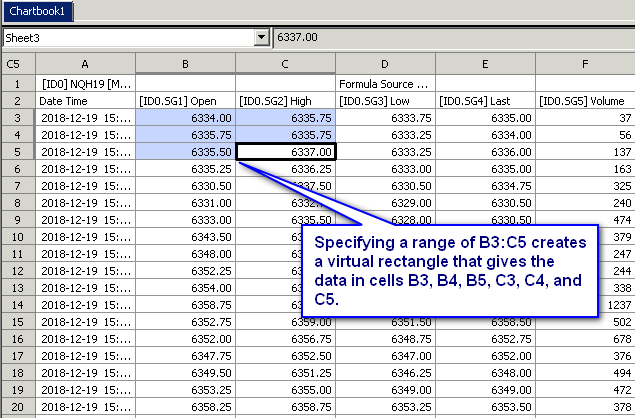
Some Spreadsheet functions can take a range of data as a parameter. This is specified when two cell references are separated by a colon (:). For these functions, the first cell reference (before the colon) specifies the upper left-hand corner of the range and the second cell reference (after the colon) specifies the lower right-hand corner of the range. This conceptual rectangle must always be drawn from upper left to lower right. As such, the row number specified by the second cell reference must always be equal to or greater than the row number specified by the first cell reference.
Specifying a range of data within a single column is well understood, as the range is easily viewable and creates a single column of data. It is, however, still necessary that the row values are increasing. For example, specifying the range B3:B5 is valid, but B5:B3 is not and will give a #REF error.
It is also possible to specify a range of data that crosses between columns. When doing this, the data that is contained with the rectangle formed from the first cell reference to the second cell reference is the range of data that will be used. For example, specifying a range of B3:C5 will include the data in the following cells: B3, B4, B5, C3, C4, and C5. As noted above, giving a range of values where the row number of the second cell reference is less than the row of the first cell reference will result in a #REF error.
Serial DateTime Values
Sierra Chart Spreadsheets store Dates and Times as double precision floating point numbers which represent the time since 1899-Dec-30 at 00:00:00. This date-time is not in any particular time zone. It can represent any time zone. To set the time zone, refer to Time Zone.
The integer part of the floating-point number represents the days and the fractional part, to the right of the decimal place, represents the time. This is exactly the same way as Excel and OpenOffice Calc represent date and Time values. This is called a Serial Date Time value.
Note that due to historical issues Excel does have a mistake in that it includes February 29, 1900, which did not exist. Therefore, Excel has 1899-12-31 as day 0 and there will be a 1 day discrepancy between Sierra Chart and Excel for dates prior to March 1, 1900.
The Spreadsheet Study, Spreadsheet System/Alert and the Spreadsheet System for Trading studies output Date-Time values to column A using this format.
Time Examples: 12 PM would be represented as .5. 1 minute or 00:01:00 would be represented as 1.0/1440.0. There are 1440 minutes in a day.
00:01:10 would be represented as 70.0/86400.0. There are 86,400 seconds in a day. 1 second evaluates to 1.15740740E-5.
Date Examples: 1900-Jan-2 would be represented as 3.
Comparing Serial Date-Time Values
Since Date-Time values are stored as floating-point numbers, they are imprecise when you are performing comparisons to them. Two Date-Time values that are the same when they are formatted as a Date and Time string, may not give you an exact comparison due to floating point error. You can see the exact values if you format the spreadsheet cell containing the Date-Time value to a number with 9 decimal places.
A solution when doing an equals comparison between 2 Date-Time values between two different sheets in the Spreadsheet, is to use a formula similar to the following: =ROUND(A3,8)=ROUND(Sheet2!A3,8) .
Sierra Chart internally stores Date-Time values in the same way as Spreadsheets do. For further information, refer to the SCDateTime data type page.
Any of the available Spreadsheet Functions which accept a Serial DateTime Value parameter or return a Serial DateTime Value can be used when working with Date-Time values in a Spreadsheet.
Using the Equivalent of COUNTIF, AVERAGEIF, MAXIF, MINIF, SUMIF
The Spreadsheets in Sierra Chart do not support the following functions: COUNTIF, AVERAGEIF, MAXIF, MINIF, SUMIF.
These are not supported due to the complexity of supporting criteria text. However, there is an alternative method to effectively perform these functions.
The Spreadsheet Studies support up to 60 formula columns. It is possible to use additional formula columns with the basic supported Spreadsheet functions to accomplish the same result as these unsupported functions.
The formula =COUNTIF(AA3:AA12,">50") can be implemented in the Sierra Chart Spreadsheets as follows:
In one of the available Spreadsheet formula columns, by default K through Z, enter this formula: =IF(AA3>50,1,0). Assuming the prior formula was entered in formula column X, then enter =SUM(X3:X12) in another formula column. The result of this last formula will be the same as =COUNTIF(AA3:AA12,">50").
Available Functions
| Format | Description |
|---|---|
| ABS(Number) (Link) | The absolute value of the given Number. If the given Number is an integer, the return value will be an integer. If the given Number value is a double, the return value will be a double. Returns #VALUE! if the given Number is not a number. |
| ACOS(Number) (Link) | The arc cosine of the given Number, in radians [0,pi]. Returns #NUM! if the given Number is outside the range of [-1,1]. Returns #VALUE! if the given Number is not a number. |
| ACOSH(Number) (Link) | Returns the inverse hyperbolic cosine of the given Number. Returns #NUM! if the given Number is less than 1. Returns #VALUE! if the given Number is not a number. |
| ADDRESS(row, column, [ref_type], [ref_style], [sheet_name]) (Link) | Returns an address represented as a text string. Returns #NUM! if row or column are less than 1.
ref_type: 1 = Absolute Row and Column. 2 = Absolute Row, Relative Column. 3 = Relative Row, Absolute Column. 4 = Relative Row and Column. |
| AND(Boolean, [...]) (Link) | Returns TRUE if and only if all of the given parameters are equal to TRUE. Otherwise, returns FALSE. Returns #VALUE! if one of the given parameters could not be interpreted as a boolean value. Examples: =AND(E3 > 10, AA3 = 100) (Spreadsheet Study formula) =AND(C > 100, SG1 < 50) (Simple Alert formula) =OR(AND(H > 100, SG1 > 100),AND(L < 80,SG1 < -100)) (Simple Alert formula) |
| ASIN(Number) (Link) | Returns the arc sine of the given Number, in radians [0,pi]. Returns #NUM! if the given Number is outside the range of [-1,1]. Returns #VALUE! if the given Number is not a number. |
| ASINH(Number) (Link) | Returns the inverse hyperbolic sine of the given Number. Returns #VALUE! if the given Number is not a number. |
| ATAN(Number) (Link) | The arc tangent of the given Number, in radians [0,pi]. Returns #VALUE! if the given Number is not a number. |
| ATANH(Number) (Link) | Returns the inverse hyperbolic tangent of the given Number. Returns #NUM! if the given Number greater or equal than 1 or less or equal that -1. Returns #VALUE! if the given Number is not a number. |
| AVEDEV(Number, [...]) (Link) | Returns the average of the absolute deviations of the numbers from their mean. Returns #VALUE! if no numbers are found. |
| AVERAGE(Number, [...]) (Link) | The average of all of the given Numbers. Null values are not counted as part of the average. Returns #NUM! if all the given Numbers are null. Returns #VALUE! if one of the Numbers given could not be interpreted as a number. |
| AVERAGE_IGNOREZEROS(Number, [...]) (Link) | The average of all of the given Numbers, except for numbers that are equal to zero. Null values are not counted as part of the average. Returns #NUM! if all the given Numbers are either null or zero. Returns #VALUE! if one of the Numbers given could not be interpreted as a number. |
| CEILING(Number, [Multiple = 1]) (Link) | Rounds the given Number up to the next number that is a multiple of the given Multiple, if the given Number does not already satisfy this condition. If Multiple is 1 or not given, the given Number is rounded up to the next whole integer. If Multiple is an integer, the returned value will be an integer, otherwise it will be a double. Returns #NUM! if the given Multiple is zero or negative. Returns #VALUE! if either the given Number or Multiple is not a number. |
| CELL(Text, [ReferenceOrRange]) (Link) | Returns information about a cell. If the first argument is "col" or "row" the column or row index is returned. If the first argument is "contents" the content of the cell is returned, if it is "type" the value type will be returned ("b" for an empty cell, "l" for a cell with constant text and "v" for other values). If the second argument is provided it is either a cell reference to return information about the referenced cell or a cell range, to return information about the first cell of a range. |
| CHOOSE(ValueNumber, Value1, [Value2, [...]]) (Link) | Returns one of the given Value arguments based on the given ValueNumber. If ValueNumber is 1, the first given Value is returned. If a cell range reference is given as a value, each of the cells within that range are treated as individual values for this function. For example, CHOOSE(3, A1:A3) will return the value of A3. Returns #REF! if the given ValueNumber is outside of the range of the values given. Returns #VALUE! if the given ValueNumber is not a number. |
| COLUMN([Reference]) (Link) | Returns the absolute (not relative) number (not index) of the column of the given Reference. If Reference is not given, then the number of the column containing this formula is returned. Returns #VALUE! if Reference is given and is not a cell reference value type. The absolute number of the first column (A) is 1. |
| COLUMNS(Range) (Link) | Returns the number of columns in the given Range. Returns #VALUE! if the given Range is not a cell range reference value type. |
| CONCATENATE(Text, [...]) (Link) | Combines the given Text values, in the order that they are given, and returns the combination as a single text value. Returns #VALUE! if one of the given parameters could not be interpreted as a text value. |
| CORREL() (Link) | See: PEARSON |
| COS(Number) (Link) | The cosine of the given number. Returns #VALUE! if the given number is not a number. |
| COSH(Number) (Link) | Returns the hyperbolic cosine of the given Number. Returns #VALUE! if the given Number is not a number. |
| COUNT([Values, [...]]) (Link) | Returns the number of numeric values given in the parameters list. If a range is given in the list, this counts the numeric values in the range. Numeric values are values that have a value type of integer or double. |
| COUNTA([Values, [...]]) (Link) | Returns the number of non-empty values given in the parameters list. If a range is given in the list, this counts the non-empty values in the range. |
| COUNTBLANK([Values, [...]]) (Link) | Returns the number of empty/blank values given in the parameter list. If a range is given in the list, this counts the empty values in the range. |
CROSSFROMABOVE(range1, range2)
|
Compares 2 ranges of values. Each range needs to contain at least 2 numbers and can contain 3 numbers. For the greatest accuracy use a range which includes 3 values with this function. Determines if the first range of values crosses the second range from above. Returns a boolean value: TRUE = The first range crosses the second Range from above. FALSE = The first range does not cross the second Range from above. If one of the range of values for the crossover needs to be a constant, then it needs to refer to a study Subgraph or formula column which contains a constant value. |
CROSSFROMBELOW(range1, range2)
|
Compares 2 ranges of values. Each range needs to contain at least 2 numbers and can contain 3 numbers. For the greatest accuracy use a range which includes 3 values with this function. Determines if the first range of values crosses the second range from below. Returns a boolean value: TRUE = The first range crosses the second Range from below. FALSE = The first range does not cross the second Range from below. If one of the range of values for the crossover needs to be a constant, then it needs to refer to a study Subgraph or formula column which contains a constant value. |
CROSSOVER(range1, range2)
|
This function compares 2 ranges of values. Each range needs to contain at least 2 numbers and can contain 3 numbers. For the greatest accuracy, use a range which includes 3 values with this function. Returns a value which indicates the type of crossing: 1 = The first Range crosses the second Range from below. -1 = The first Range crosses the second Range from above. 0 = The ranges do not cross each other. If one of the range of values for the crossover needs to be a constant, then it needs to refer to a study Subgraph or formula column which contains a constant value. |
| DATE(Year, Month, Day) (Link) | Returns a Serial DateTime Value for the given Year, Month, and Day. Returns #NUM! if the given Year, Month, and Day does not specify a valid day. Returns #VALUE! if any of the parameters could not be interpreted as integer values. |
| DATEVALUE(Text) (Link) | Returns a Serial DateTime Value for the given Text, interpreted as a date string. The Text must be given in the form "m/d/YYYY" including quotes, where m is the numerical month (one or two digits), d is numerical day (one or two digits) and YYYY is the year - For example "3/22/2018". Returns #NUM! if the given Text cannot be interpreted as a valid date. Returns #VALUE! if the given Text cannot be interpreted as text value. |
| DAY(Serial DateTime Value) (Link) | Returns the day of the month for the given serial date-time value. 1 is returned for the first day of the month. Returns #VALUE! if the given DateTime cannot be interpreted as a serial date value. |
| DAYS360() (Link) | Returns the number of days between the start date and the end date using a 360-day year, 30 day month calendar that is used in accounting systems. |
| DEVSQ(Numbers, [...]) (Link) | Returns the sum of the squares of deviations from the average. Returns #VALUE! if no numbers are found. |
| DEGREES(Radians) (Link) | Converts the given Radians into degrees about a unit circle. Returns #VALUE! if the given Radians is not a number. |
| EARLIESTNONZEROVALUE(Range) (Link) | Returns the last non-zero value in the given Range. Empty cells are considered equivalent to zero. Returns a null value if all of the values in the Range are either null or zero. |
| EDATE(Date, Months) (Link) | Returns the serial date that is the given number of Months after the specified Date. If Months is less than 0, the return value is the date that is the indicated number of months before the given Date. If the same day of the month does not exist in the resulting month, then the last day of the resulting month is returned. Returns #VALUE! if the arguments are not integers. |
| EOMONTH(Date, Months) (Link) | Returns the serial date number of the last day of the month that is a number of months after the specified date. If the second argument is less than 0, the return value is the date that is the last day of the month the indicated number of months before the date. Returns #VALUE! if the arguments are not integers. |
| EVEN(Number) (Link) | If the number is not even, rounds it up to the next even number. If the Number is less than 0 it will be rounded away from 0. Returns #VALUE! if the argument is not a number. |
| EXP(Number) (Link) | Returns the value of e (mathematical constant) raised to the given Number. Returns #VALUE! if the given Number is not a number. |
| FIND(SubString, FullString, [StartPosition = 1]) (Link) | Returns the starting position of the first instance of the given SubString text within the given FullString text. The return value is 1-based, meaning if the given SubString is found at the very beginning of the given FullString, the return value will be 1. By default, FIND begins the search for the given SubString at the beginning of the given FullString, but this can be moved by specifying a value greater than 1 for the optional StartPosition parameter. The search is case-sensitive (use SEARCH for a case-insensitive search). Returns 1 if the given SubString is empty. Returns #VALUE! if no match is found, or the given StartPosition is beyond the length of the given FullString, or one of the strings is not a text value, or the given StartPosition is not an integer value. Returns #NUM! if the given StartPosition is less than 1. |
| FISHER(Number) (Link) | Returns the Fisher Transformation for a given number. Returns #NUM! if the Number is less than or equal to -1, or greater than or equal to 1. Returns #VALUE! if the argument is not a number. |
| FISHERINV(Number) (Link) | Returns the Inverse Fisher Transformation for a given number. Returns #VALUE! if the argument is not a number. |
| FLOOR(Number, [Multiple = 1]) (Link) | Rounds the given Number down to the next number that is a multiple of the given Multiple, if the given Number does not already satisfy this condition. If Multiple is 1 or not given, the given Number is rounded down to the next whole integer. If Multiple is an integer, the returned value will be an integer, otherwise it will be a double. Returns #NUM! if the given Multiple is zero or negative. Returns #VALUE! if either the given Number or Multiple is not a number. |
| FORECAST(X, KnownYs, KnownXs) (Link) | Returns a predicted value using linear regression based on the known X and known Y values. Refer to Using the FORECAST Function for more information. |
| FRACTIME(DateTime) (Link) | Returns the fractional time part of the given DateTime value. Returns 0 if the given DateTime value is empty. Returns #VALUE! if the given DateTime cannot be interpreted as a serial date-time value. |
| GetCorrespondingMatch(SearchColumn, SearchValue, NearestOrExact, SearchRangeOrderingFlag, SameValueResolution, ReturnResultColumn, ReturnResultRowOffset) (Link) |
Searches a range of values for the SearchValue and returns a reference to the corresponding cell at the same found row index, or an offset, in another column range. SearchColumn: The column range to be searched. Example: AA3:AA102. SearchValue: The value to search for in the SearchColumn. Only doubles, integers and TRUE/FALSE are supported. Specifying a text value returns an error. Searching for text is not supported. Any value given for SearchValue that cannot be interpreted as a double, integer or TRUE/FALSE value results in a #VALUE! error. Example: 50.0. NearestOrExact: 0 = exact match. 1 = nearest match. While iterating through the ordered elements, and an exact match cannot be found and the NearestOrExact parameter is set to 1, the nearest match will instead be returned. Example: 0. SearchRangeOrderingFlag: 1 = SearchColumn values are ascending. (Lowest numbered row has the lowest numbers. Highest numbered row has higher numbers).
SameValueResolution: When there are values which repeat within an ordered SearchColumn, this parameter indicates how to resolve that. 1 = Use higher numbered row index. 0 = Use lower numbered row index. Example: 0. ReturnResultColumn: The column range where a reference will be returned for the corresponding row where the match was found. This parameter can be the same as SearchColumn. Example: AA3:AA102. ReturnResultRowOffset: A positive or negative row offset for the row returned by ReturnResultColumn. Example: 0. Example: = GetCorrespondingMatch(AA$3:AA$402, 9, 1, 0, 0, AA$3:AA$402, 0) |
| HLOOKUP(Value, Range, RowInRange, [ApproximateMatch]) (Link) | Searches for the given Value in the top-most row of the given Range, and returns a reference the the cell at the same column of the found value, at the row at the given RowInRange.
RowInRange is a row index within the given Range, where 1 is the top-most row of the given Range. If ApproximateMatch is given as TRUE, and no exact match is found, the last value within the given Range that is less than the given Value will be used. When ApproximateMatch is given as TRUE, the values in the top-most row of the given Range are assumed to be in ascending order. If ApproximateMatch is not given or given as FALSE and the given Value is not found, #N/A! is returned. Returns #VALUE! if the given Value cannot be resolved to an actual value (such as if a range reference is given), or the given RowInRange cannot be interpreted as an integer value, or the given ApproximateMatch cannot be interpreted as a boolean value. Returns #REF! if the given Range is not valid, or the given RowInRange is beyond the number of rows in the given Range. Returns #NUM! if the given RowInRange is less than 1. |
| HOUR(Serial DateTime Value) (Link) | Returns the hour for the given Serial DateTime Value. This function will return values in the range 0-23. Returns #VALUE! if the given DateTime cannot be interpreted as a serial date-time value. |
| HULL_INTERMEDIATE(Reference, Value) (Link) | Returns the Intermediate calculation values for the Hull Moving Average. This is meant to be used in combination with the HULL_RESULT function, with this function in one column and the HULL_RESULT function in another column. The Reference is to the first (top) cell of the data and the Value defines the length of the Moving Average (the number of cells to include). The Value used in this function needs to match the value used in the HULL_RESULT function. Empty cells are considered to have a value of 0. Returns #VALUE if the first parameter is not a reference to a cell, or if the second parameter is not an integer, or if any of the values within the input range is not a number. Returns #NUM if the Value parameter is not large enough for a complete calculation. |
| HULL_RESULT(Reference, Value) (Link) | Returns the final calculation values for the Hull Moving Average. This is meant to be used in combination with the HULL_INTERMEDIATE function, with this function in one column and the HULL_INTERMEDIATE function in another column. The Reference is to the first (top) cell of the HULL_INTERMEDIATE column and the Value defines the length of the Moving Average (the number of cells to include). The Value used in this function needs to match the value used in the HULL_INTERMEDIATE function. Empty cells are considered to have a value of 0. Returns #VALUE if the first parameter is not a reference to a cell, or if the second parameter is not an integer, or if any of the values within the input range is not a number. Returns #NUM if the Value parameter is not large enough for a complete calculation. |
| IF(Condition, TrueValue, FalseValue) (Link) | Returns the value of TrueValue if the given Condition is equal to TRUE. Returns the value of FalseValue if the given Condition is equal to FALSE. Returns #VALUE! if the condition could not be interpreted as a boolean value.
Multiple IF statements can be strung together to create a series of IF/ELSE IF functions. To do this, simply put additional IF statements for the FalseValue arguments. For example: IF(A > B, 1, IF(B > C, 2, 0)). This would evaluate as: if A is greater than B then 1, else if B is greater than C then 2, else 0. |
| INDEX(Range, Index) or INDEX(Range, Row, Column) (Link) | Returns a cell reference within the given Range, either at the given Index or the given Row and Column within the Range. If using Index (only one parameter after Range) on a Range with multiple rows and columns, the items are ordered down by rows first, and then across by columns.
Index, Row, and Column are all 1-based, meaning using a value of 1 will return the first value. Returns #REF! if the given Index, Row, or Column is outside of the given Range. Returns #VALUE! if the given Range is not a cell reference range type, or if the given Index, Row, or Column could not be interpreted as integer values. |
| INDIRECT(ReferenceText) (Link) | Returns a reference specified by the given ReferenceText. The ReferenceText must be a text value that can be parsed as a standard reference as used in formulas. This function only supports basic cell references, basic cell range references, and basic column range references; advanced references are not supported. Returns a #REF! error if the given ReferenceText cannot be parsed or is otherwise invalid. Returns #VALUE! if the given ReferenceText is not a text value.
An example ReferenceText is "E3". ReferenceText can be created by a formula. For example, if cell H5 contains the number 3, then the following formula will return E3: CONCATENATE("E", H5). |
| INT(Number) (Link) | Rounds the given Number down to the next whole integer. Returns #VALUE! if the given Number is not a number. Returns 0 if Number is an empty value, like a reference to a cell that contains no data. |
| INTDATE(DateTime) (Link) | Returns the integer date part of the given DateTime value. Returns 0 if the given DateTime value is empty. Returns #VALUE! if the given DateTime cannot be interpreted as a serial date-time value. |
| ISBLANK(Value) (Link) | Returns TRUE if the given Value is blank, which means no value type. Otherwise returns FALSE. |
| ISEMPTY(Value) (Link) | Returns TRUE if the given Value is empty, which means no value type. Otherwise returns FALSE. |
| ISERR(Value) (Link) | Returns TRUE if the given Value is an error value type. Otherwise returns FALSE.
IFERROR(A, B, C) can be written as IF(ERR(A), B, C). IFNA(A, B, C) can be written as IF(A=#N/A, B, C). |
| ISEVEN(Number) (Link) | Returns TRUE if the given Number is an even number. Otherwise returns FALSE. If the given Number is a double value, only the integer part is checked. Returns #VALUE! if the given Number is not a number. |
| ISLOGICAL(Value) (Link) | Returns TRUE if the given Value is a boolean value type. Otherwise returns FALSE. |
| ISNULL(Number) (Link) | Returns TRUE if the given Value is null, which means no value type. Otherwise returns FALSE. |
| ISNUMBER(Number) (Link) | Returns TRUE if the given Value is an integer or double value type. Otherwise returns FALSE. |
| ISODD(Number) (Link) | Returns TRUE if the given Number is an odd number. Otherwise returns FALSE. If the given Number is a double value, only the integer part is checked. Returns #VALUE! if the given Number is not a number. |
| ISRANGE(Value) (Link) | Returns TRUE if the type of the given Value is a range type. Otherwise returns FALSE. |
| ISREF(Value) (Link) | Returns TRUE if the type of the given Value is a reference type. Otherwise returns FALSE. |
| ISSAMETIMETOHOUR(DateTime1, DateTime2) (Link) | Returns TRUE if the time values for both of the given serial date-time values are at the same time, down to the hour. Example: comparing 12:00:00.000 to 12:59:59.999 would return TRUE, but comparing 12:59:59.999 to 13:00:00.000 would return FALSE. The date component of both values is ignored. Returns #VALUE! if either of the given values cannot be interpreted as a serial date-time value. |
| ISSAMETIMETOMILLISECOND(DateTime1, DateTime2) (Link) | Returns TRUE if the time values for both of the given serial date-time values are at the same time, down to the millisecond. Example: comparing 12:00:00.000 to 12:00:00.000 would return TRUE, but comparing 12:00:00.000 to 12:00:00.001 would return FALSE. The date component of both values is ignored. Returns #VALUE! if either of the given values cannot be interpreted as a serial date-time value. |
| ISSAMETIMETOMINUTE(DateTime1, DateTime2) (Link) | Returns TRUE if the time values for both of the given serial date-time values are at the same time, down to the minute. Example: comparing 12:00:00.000 to 12:00:59.999 would return TRUE, but comparing 12:00:59.999 to 12:01:00.000 would return FALSE. The date component of both values is ignored. Returns #VALUE! if either of the given values cannot be interpreted as a serial date-time value. |
| ISSAMETIMETOSECOND(DateTime1, DateTime2) (Link) | Returns TRUE if the time values for both of the given serial date-time values are at the same time, down to the second. Example: comparing 12:00:00.000 to 12:00:00.999 would return TRUE, but comparing 12:00:00.999 to 12:00:01.000 would return FALSE. The date component of both values is ignored. Returns #VALUE! if either of the given values cannot be interpreted as a serial date-time value. |
| ISTEXT(Value) (Link) | Returns TRUE if the given Value is a text value type. Otherwise returns FALSE. |
| LARGE(Numbers, NthLargest) (Link) | Returns the Nth largest number from an array of numbers. The first argument is the array, while the last argument controls which number will be returned. 1 means the largest number, 2 the second largest and so on.
Empty cells are not counted, TRUE will be considered as 1, FALSE as 0. Returns #VALUE! if the last argument is larger than 1 or greater than the number of numerical values (and booleans) in the array. |
| LEN(Text) (Link) | Returns the number of characters in the given Text string. Returns #VALUE! if Text is not a string. |
| LEFT(Text, Count) (Link) | Returns the given Count number of characters from left side of the given Text string. If Count is greater than the length of the given Text string, then the entire string will be returned. If Count is 0, an empty string is returned. If the given Count is negative, then the entire length of the given Text string, except for -Count characters, will be returned. Returns #VALUE! if Text is not a string, or Count is not an integer. |
| LN(Number) (Link) | Returns the natural logarithm (using base e) of the given Number. Returns #NUM! if the given Number is less than or equal to 0. Returns #VALUE! if the given Number is not a number. |
| LOG(Number, [Base = 10]) (Link) | Returns the logarithm of the given Number using the given Base. If Base is not given, the base defaults to 10. Returns #NUM! if either the given Number or Base is less than or equal to 0. Returns #VALUE! if either the given Number or Base is not a number. |
| LOG10(Number) (Link) | Returns the logarithm of the given Number using base 10. Returns #NUM! if the given Number is less than or equal to 0. Returns #VALUE! if the given Number is not a number. |
| MATCH(Number, Range, [MatchType]) (Link) | It is strongly recommended to use the new GetCorrespondingMatch function which is highly optimized and has performance 90% faster than MATCH.
Searches an array/range for Number using MatchType as the comparison method, and returns the one-based index into this array/range of numbers indicating the position of the match. Returns #N/A! if no match is found. MatchType: This is optional and the default value is 0. It can be one of the following:
|
| MAX(Numbers, [...]) (Link) | Returns the number with the maximum value out of all the given Numbers. Returns #VALUE! if one of the given Numbers could not be interpreted as a number. |
| MAXL(Value, Numbers, [...]) (Link) | Returns the number with the maximum value out of all the given Numbers that is less than the given Value. Returns #VALUE! if the given Value or one of the given Numbers could not be interpreted as a number. |
| MEDIAN(Numbers, [...]) (Link) | The median value of all of the given Numbers. Null values are not counted as part of the median. No value is returned if all the given Numbers are null. Returns #VALUE! if one of the Numbers given could not be interpreted as a number. |
| MID(Text, Offset, Count) (Link) | Returns the text string from the middle of the given Text string, starting at the given Offset, and including the given Count number of characters. If Offset is 0, the result will start at the beginning of the string. If Offset + Count is greater than the length of the given Text string, the returned text will go up to the end of the given Text string. If Count is 0, or Offset is greater than or equal to the length of the sting, an empty string will be returned. Returns #NUM! if the given Offset or Count is negative. Returns #VALUE! if Text is not a text value, or if Offset or Count could not be interpreted as integer values. |
| MILLISECOND(Serial DateTime Value) (Link) | Returns the millisecond for the given Serial DateTime Value. This function will return values in the range 0-999. Returns #VALUE! if the given DateTime cannot be interpreted as a serial date-time value. |
| MIN(Numbers, [...]) (Link) | Returns the number with the minimum value out of all the given Numbers. Returns #VALUE! if one of the given Numbers could not be interpreted as a number. |
| MING(Value, Numbers, [...]) (Link) | Returns the number with the minimum value out of all the given Numbers that is greater than the given Value. Returns #VALUE! if the given Value or one of the given Numbers could not be interpreted as a number. |
| MINUTE(Serial DateTime Value) (Link) | Returns the minute for the given Serial DateTime Value. This function will return values in the range 0-59. Returns #VALUE! if the given DateTime cannot be interpreted as a serial date-time value. |
| MINZ(Numbers, [...]) (Link) | Returns the number with the minimum value out of all the given Numbers that is greater than zero. Returns #VALUE! if one of the given Numbers could not be interpreted as a number. |
| MOD(Number, Divisor) (Link) | The remainder of the given Number divided by the given Divisor. Returns #DIV/0! if the given Divisor is 0. Calculates the return value using the formula Number - Divisor * INT(Number/Divisor) that gives the result when the arguments are not integers. |
| MODE(Values, [...]) (Link) | Returns the value that occurs most frequently among the given Values. Returns the first value in the order given if multiple different values are tied for the most frequent occurrence. Returns #N/A if there are no values that occur more than once. Empty values are not counted. This function works with both numeric and text values, but if there is an error value among the given values, the first error value is returned. |
| MONTH(DateTime) (Link) | Returns the month for the given Serial DateTime Value. 1 is returned for the first month of the year (January). Returns #VALUE! if the given DateTime cannot be interpreted as a serial date value. |
| MOSTRECENTNONZEROVALUE(Range) (Link) | Returns the first non-zero value in the given Range. Empty cells are considered equivalent to zero. Returns a null value if all of the values in the Range are either null or zero. |
| MROUND(Number, Multiple) (Link) | Rounds the given Number to the nearest number that is a multiple of the given Multiple, if the given Number does not already satisfy this condition. If Multiple is 1, the given Number is rounded to the nearest whole integer. If Multiple is an integer, the returned value will be an integer, otherwise it will be a double. Returns #NUM! if the given Multiple is zero or negative. Returns #VALUE! if either the given Number or Multiple is not a number. |
| MROUNDDOWN() (Link) | Refer to FLOOR. |
| MROUNDUP() (Link) | Refer to CEILING. |
| NETWORKDAYS(StartDate, EndDate, [Holidays]) (Link) | Returns work days between the given StartDate and EndDate, including both the StartDate and the EndDate, not counting weekends or the specified Holidays. |
| NMATCH(N, Value, Range, [MatchType]) (Link) | Same as MATCH, except the search continues until the Nth matching item is found, where N is a positive integer. Searches the given Range for the given Value using MatchType as the comparison method. Returns a one-based index into the given Range indicating the position of the match. Returns #N/A! if N matches were not found.
MatchType: This is optional and the default value is 0. It can be one of the following:
|
| NORM.DIST(X, Mean, StdDev, Cumulative) (Link) | Computes the the Normal Distribution for X, Mean, and StdDev. If Cumulative is set to 1, the function returns the value of the Cumulative Distribution Function (CDF). If Cumulative is set to 0, the function returns the value of the Probability Distribution Function (PDF). |
| NORM.S.DIST(X, Cumulative) (Link) | Computes the Standard Normal Distribution for X (with Mean 0 and StdDev 1). If Cumulative is set to 1, the function returns the value of the Cumulative Distribution Function (CDF). If Cumulative is set to 0, the function returns the value of the Probability Distribution Function (PDF). |
| NOW() (Link) | Returns the current local date and time as a Serial DateTime Value. The serial date-time value 2.0 represents 00:00:00 (midnight), January 1st, 1900, and 2.5 represents 12:00:00 (noon) for that same day. |
| ODD(Number) (Link) | If the number is not odd, rounds it up to the next odd number. If the Number is less than 0 it will be rounded away from 0. Returns #VALUE! if the argument is not a number. |
| OFFSET(From, Rows, Columns, [Height], [Width]) (Link) | Returns the reference or the cell range calculated from a reference or a cell range (passed as the first argument) and some offset values. |
| OR(Boolean, [...]) (Link) | Returns FALSE if and only if all of the given parameters are equal to FALSE. Otherwise returns TRUE. Returns #VALUE! if one of the given parameters could not be interpreted as a boolean value. Examples: =OR(E3 < 10, E3 > 15) (Spreadsheet Study formula) =OR(SG1 > 40, SG1 < 20) (Simple Alert formula) =OR(AND(H > 100, SG1 > 100),AND(L < 80,SG1 < -100)) (Simple Alert formula) |
| PEARSON(Array1, Array2) (Link) | Returns the Pearson product moment correlation coefficient between -1.0 and 1.0. Returns #VALUE! if the size of the arrays are not equal or the arrays are empty. Returns #DIV/0! for certain arrays. |
| PERCENTILE(Numbers, K) (Link) | Returns the K-th percentile of values in a cell range. Uses linear interpolation between values if K is not a multiple of 1 / (n - 1), where n is the number of the numerical values found in the cell range. Returns #VALUE! if K is not a number. Returns #NUM! if K is less than 0 or greater than 1. |
| PERCENTRANK(Array, X, [Significance]) (Link) | Returns the rank of a value in a data set as a percentage of the data set size. If the value can be found in between two values of the set, the return value will be calculated by linear interpolation. Returns #VALUE! if the number is less than the smallest or greater than the biggest number. Returns #NUM! if the array is empty. If the third argument is provided it will control how many digits will be used to compare values. If the third argument is less than 1 the #NUM! error will be returned. |
| PROB(Values, Probability, LowerLimit, [UpperLimit]) (Link) | Calculates the probability that values in a range are between two limits. If the upper limit is omitted calculates the probability that values in the range are equal to the lower limit. If the Numbers and the Probabilities contain different number of data points the function will return #N/A error. If any probability value is less or equal to 0 or greater than 1.0 the function will return #NUM! error. If the total of the probability is not 1.0 the functions returns #NUM! error. |
| RADIANS(Degrees) (Link) | Converts the given Degrees into radians about a unit circle. Returns #VALUE! if the given Degrees is not a number. |
| RAND() Or RAND(Low, High) (Link) | Generates a random decimal number. If no arguments are given, returns a random decimal number from 0.0 to 1.0. Returns #ARGS! if only one argument is given. If the two arguments Low and High are given, returns a random decimal number from Low to High. Returns #NUM! if Low is greater than High. Returns #VALUE if the given Low or High could not be interpreted as numbers. |
| RANDINT() Or RANDINT(Low, High) (Link) | Generates a random integer number. If the single argument Count is given, returns a randomly selected integer from 1 to Count. Returns #NUM! if Count is less than 1. If the two arguments Low and High are given, returns a randomly selected integer from Low to High. Returns #NUM! if Low is greater than High. Returns #VALUE! if Count, Low, or High could not be interpreted as integer values. |
| RIGHT(Text, Count) (Link) | Returns the given Count number of characters from right side of the given Text string. If Count is greater than the length of the given Text string, then the entire string will be returned. If Count is 0, an empty string is returned. If the given Count is negative, then the entire length of the given Text string, except for -Count characters, will be returned. Returns #VALUE! if Text is not a string, or Count is not an integer. |
| ROUND(Number, [Digits = 0]) (Link) | Rounds the given Number to the nearest number with the number of given Digits. If Digits is 0 or not given, the given Number is rounded to the nearest whole integer. If Digits is positive, the given Number is rounded to the nearest number with that many decimal digits. Example: ROUND(1.235,1) = 1.2; ROUND(1.235,2) = 1.24. If Digits is negative, the given Number is rounded to the nearest number that is a multiple of 10^(-Digits). Example: ROUND(1235, -1) = 1240; ROUND(1235, -2) = 1200. If Digits >= 0, the returned value will be an integer, otherwise it will be a double. Returns #VALUE! if the given Number is not a number, or if the given Digits (when given) is not an integer. |
| ROUNDDOWN(Number, [Digits = 0]) (Link) | Rounds the given Number down to the next number with the number of given Digits, if the given Number does not already satisfy this condition. Rounding down means closer to 0, so a positive number rounded down will be less than or equal to the given Number, and a negative number rounded down will be greater than or equal to the given Number. If Digits is 0 or not given, the given Number is rounded down to the next whole integer. If Digits is positive, the given Number is rounded down to the next number with that many decimal digits. Example: ROUNDDOWN(1.235,1) = 1.2; ROUNDDOWN(1.235,2) = 1.23. If Digits is negative, the given Number is rounded down to the next number that is a multiple of 10^(-Digits). Example: ROUNDDOWN(1235, -1) = 1230; ROUNDDOWN(1235, -2) = 1200. If Digits >= 0, the returned value will be an integer, otherwise it will be a double. Returns #VALUE! if the given Number is not a number, or if the given Digits (when given) is not an integer. |
| ROUNDUP(Number, [Digits = 0]) (Link) | Rounds the given Number up to the next number with the number of given Digits, if the given Number does not already satisfy this condition. Rounding up means farther away from 0, so a positive number rounded up will be greater than or equal to the given Number, and a negative number rounded up will be less than or equal to the given Number. If Digits is 0 or not given, the given Number is rounded up to the next whole integer. If Digits is positive, the given Number is rounded up to the next number with that many decimal digits. Example: ROUNDUP(1.235,1) = 1.3; ROUNDUP(1.235,2) = 1.24. If Digits is negative, the given Number is rounded up to the next number that is a multiple of 10^(-Digits). Example: ROUNDUP(1235, -1) = 1240; ROUNDUP(1235, -2) = 1300. If Digits >= 0, the returned value will be an integer, otherwise it will be a double. Returns #VALUE! if the given Number is not a number, or if the given Digits (when given) is not an integer. |
| ROW([Reference]) (Link) | Returns the absolute (not relative) number (not index) of the row of the given Reference. If Reference is not given, then the number of the row containing this formula is returned. Returns #VALUE! if Reference is given and is not a cell reference value type. The absolute number of the first row (1) is 1. |
| ROWS(Range) (Link) | Returns the number of rows in the given Range. Returns #VALUE! if the given Range is not a cell range reference value type. |
| SEARCH(SubString, FullString, [StartPosition = 1]) (Link) | Returns the starting position of the first instance of the given SubString text within the given FullString text. The return value is 1-based, meaning if the given SubString is found at the very beginning of the given FullString, the return value will be 1. By default, SEARCH begins the search for the given SubString at the beginning of the given FullString, but this can be moved by specifying a value greater than 1 for the optional StartPosition parameter. The search is case-insensitive (use FIND for a case-sensitive search). Returns 1 if the given SubString is empty. Returns #VALUE! if no match is found, or the given StartPosition is beyond the length of the given FullString, or one of the strings is not a text value, or the given StartPosition is not an integer value. Returns #NUM! if the given StartPosition is less than 1. |
| SECOND(Serial DateTime Value) (Link) | Returns the second for the given Serial DateTime Value. This function will return values in the range 0-59. Returns #VALUE! if the given DateTime cannot be interpreted as a serial date-time value. |
| SIGN(Number) (Link) | Returns 1 if the given Number is positive, -1 if the given Number is negative, or 0 if the given Number is zero. Returns #VALUE! if the given Number is not a number. |
| SIN(Number) (Link) | The sine of the given number. Returns #VALUE! if the given number is not a number. |
| SINH(Number) (Link) | Returns the hyperbolic sine of the given Number. Returns #VALUE! if the given Number is not a number. |
| SLOPE(KnownYs, KnownXs) (Link) |
Returns the slope of the linear regression line through a set of known X and Y values. The first parameter is a reference to a range of cells containing the known Y values, and the second parameter is a reference to a range of cells containing the known X values. Only numeric values in the given ranges will be used. Returns #NUM! if the number of known X and Y values do not match. Returns #DIV/0! if no numeric values are given, or the slope is vertical. Example: |
| SMALL(Numbers, NthSmallest) (Link) | Returns the Nth smallest number from an array of numbers. The first argument is the array, while the last argument controls which number will be returned. 1 means the smallest number, 2 the second smallest and so on. Empty cells are not counted, TRUE will be considered as 1, FALSE as 0. Returns #VALUE! if the last argument is smaller than 1 or greater than the number of numerical values (and booleans) in the array. |
| SQRT(Numbers) (Link) | The square root of the given Number. Returns #NUM! if the given Number is negative. Returns #VALUE! if the given Number is not a number. |
| STANDARDIZE(X, Mean, StandardDev) (Link) | Returns the normalized value from a distribution characterized by the given Mean and StandardDev. The equation for the normalized value is [ (X - Mean) / StandardDev ]. Returns #NUM! if the given StandardDev is less than or equal to 0. |
| STDEV(Numbers, [...]) (Link) | Refer to STDEV.S. |
| STDEV.P(Numbers, [...]) (Link) | Returns the standard deviation of a population. Empty values are ignored. Returns #VALUE! if one of the Numbers could not be interpreted as a number, or if there are fewer than 2 numbers in the arguments. |
| STDEV.S(Numbers, [...]) (Link) | Returns the standard deviation of a sample. Empty values are ignored. Returns #VALUE! if one of the Numbers could not be interpreted as a number, or if there are fewer than 2 numbers in the arguments. For the formula used, refer to STDEV. |
| SUM(Numbers, [...]) (Link) | The total of all the numbers given added together. If all the given Numbers are integer values, then the result will be an integer value. Otherwise the result will be a double value. Returns #VALUE! if one of the given Numbers could not be interpreted as a number. |
| SUMPRODUCT(Range1, [Range2, ...]) (Link) | Multiplies the corresponding cell values in all of the given ranges, and then returns the sum of those products. For example, if three ranges are given, the values of the first cells in all three ranges will be multiplied together; that product will be added to the product of the second cell in all three ranges, and so on until the last cell of all three ranges. Any cells that do not contain a numeric value are treated as having a value of zero. Returns #VALUE! if any of the arguments are not cell range reference. Returns #NUM! if all the ranges do not have the same number of cells. |
| TAN(Numbers) (Link) | The tangent of the given number. Returns #VALUE! if the given number is not a number. |
| TANH(Numbers) (Link) | The hyperbolic tangent of the given number. Returns #VALUE! if the given number is not a number. |
| TEXT(Value, Format) (Link) | Returns the given Value as a text value. The given Format text is used for formatting numeric values. It is optional and has no effect on other value types.
To format a number with a specific number of decimal places, use a format such as ".000" or ".###". For each "0" following the decimal point in the Format, that many decimal points will be displayed, even if they are insignificant. For example: TEXT(0.05, "0.000") will return "0.050". For each number sign (#) following the decimal point in the Format, that many decimal points will be displayed, except for trailing zeros. For example: TEXT(0.05, "0.###") will return "0.05". These two methods can be combined such that ".00##" will format numbers with a minimum of two decimal digits and a maximum of four decimal digits. Values will be rounded to the maximum number of decimal digits that can be shown. Zeros placed before the decimal point indicate to use leading zeros for the whole number. For example: TEXT(2.5, "000.##") will return "002.5". Number signs (#) before the decimal point have no effect. The decimal point in the Format text must match the global setting that specifies the decimal point character. The decimal point character used in the returned value will match the global setting. |
| TIME(Hour, Minute, Second, [Millisecond = 0]) (Link) | Returns a Serial DateTime Value for the given Hour, Minute, Second, and Millisecond. If Millisecond is not given, a value of 0 is used for the millisecond portion. Returns #NUM! if the given Hour, Minute, Second, and Millisecond does not specify a valid time. Returns #VALUE if any of the parameters cannot be interpreted as integer values.
Here is an example of a formula to use in one of the formula columns at Sheet row 3 which returns TRUE(1) when the time value in the Date-Time column of the Sheet used by the Spreadsheet Study at the corresponding row is between the times 9:30:00 and 9:34:59 =AND(FRACTIME(A3)>=TIME(9, 29, 59, 750), FRACTIME(A3)<TIME(9, 34, 59, 250)) Milliseconds are used to make this an accurate comparison due to floating-point error. |
| TIMEVALUE(Text) (Link) | Returns a Serial DateTime Value for the given Text, interpreted as a time string. Returns #NUM! if the given Text cannot be interpreted as a valid time. Returns #VALUE if the given Text cannot be interpreted as text value. |
| TODAY() (Link) | Returns the current local date as a Serial DateTime Value. A serial date value is the number of days since 1899-12-30 (day 0). The serial date value for January 1st, 1900 is 2. |
| TRIMMEAN(Range, Percent) (Link) | Sorts the values in the given Range, and returns the average of the inner values, excluding a percentage of the outer values (the extremes). The number of excluded values is equal to the number of values in the range, multiplied by the given Percent, rounded down to the nearest multiple of 2.
This way an equal number of values will be excluded from both the high and the low end of the range of values. Cells with no value are not counted as part of the values in the range. Returns #NUM! if there are either no values to average, or the given Percent is less than zero or greater than one. Returns #VALUE! if the given Range contains any non-numeric values. |
| TRUNC(Number, [Digits = 0]) (Link) | Returns the given Number truncated to the given number of Digits. If the given number of Digits is 0 or not specified, then the Number is truncated to a whole number. If the given number of Digits is greater than 0, then the given Number is truncated to that many decimal digits. If the given number of Digits is less than 0, then the given Number is truncated to the multiple of 10^(-Digits). Returns #VALUE! if the given Number is not a number, or the given Digits is not an integer. |
| TRUNCHOUR(DateTime, [Hours = 1]) (Link) | Returns the given DateTime truncated down to the exact hour. If Hours is greater than 1, the given DateTime is truncated down to the interval of the given Hours (e.g. 2 hours, 3 hours, etc.). Returns #NUM! if the given Hours is less than 1. Returns #VALUE! if the given DateTime is not a number, or the given Hours is not an integer. |
| TRUNCMIN(DateTime, [Minutes = 1]) (Link) | Returns the given DateTime truncated down to the exact minute. If Minutes is greater than 1, the given DateTime is truncated down to the interval of the given Minutes (e.g. 5 minutes, 10 minutes, etc.). Returns #NUM! if the given Minutes is less than 1. Returns #VALUE! if the given DateTime is not a number, or the given Minutes is not an integer. |
| TRUNCSEC(DateTime, [Seconds = 1]) (Link) | Returns the given DateTime truncated down to the exact second. If Seconds is greater than 1, the given DateTime is truncated down to the interval of the given Seconds (e.g. 5 seconds, 10 seconds, etc.). Returns #NUM! if the given Seconds is less than 1. Returns #VALUE! if the given DateTime is not a number, or the given Seconds is not an integer. |
| TYPE(Argument) (Link) | Returns the type of an argument encoded as an integer. Empty cells considered to have a numerical value returning 1. Return values:
1 = Number 2 = Text string 4 = Logical value 16 = Error value 64 = Cell range |
| VALUE(Text) (Link) | Converts the given Text into a number. Returns #VALUE! if the text cannot be properly converted into a number. If a numeric value type is given for the Text, that value is simply returned. |
| VLOOKUP(Value, Range, ColumnInRange, [ApproximateMatch]) (Link) | Searches for the given Value in the left-most column of the given Range, and returns a reference the the cell at the same row of the found value, at the column at the given ColumnInRange.
ColumnInRange is a column index within the given Range, where 1 is the left-most column of the given Range. If ApproximateMatch is given as TRUE, and no exact match is found, the last value within the given Range that is less than the given Value will be used. When ApproximateMatch is given as TRUE, the values in the left-most column of the given Range are assumed to be in ascending order. If ApproximateMatch is not given or given as FALSE and the given Value is not found, #N/A! is returned. Returns #VALUE! if the given Value cannot be resolved to an actual value (such as if a range reference is given), or the given ColumnInRange cannot be interpreted as an integer value, or the given ApproximateMatch cannot be interpreted as a boolean value. Returns #REF! if the given Range is not valid, or the given ColumnInRange is beyond the number of columns in the given Range. Returns #NUM! if the given ColumnInRange is less than 1. |
| WEEKDAY(Serial DateTime Value) (Link) | Returns an integer representing the day of the week for the given Serial DateTime Value. The return value will be in the range of 1-7 (1=Sunday, 7=Saturday). Returns #VALUE! if the given DateTime cannot be interpreted as a serial date value. |
| WEEKNUM(Serial DateTime Value) (Link) | Returns an integer representing the week number that contains the given Serial DateTime Value. The return value will be in the range of 1-53. A date of January 1st of any given year will always return a value of 1. Subsequent weeks start at midnight on Sunday. Returns #VALUE! if the given DateTime cannot be interpreted as a serial date value. |
| WEIGHTEDMOVINGAVERAGE(Range) (Link) | Returns the Weighted Moving Average of the inputted Range of values. Returns #VALUE! if the given range of data does not contain numeric values. Refer to Moving Average - Weighted for information on the calculation. |
| WORKDAY(StartDate, WorkDays, [Holidays]) (Link) | Returns the serial date that is the given number of WorkDays before or after the given StartDate. Work days exclude weekends and any given Holidays. |
| YEAR(DateTime) (Link) | Returns the year for the given Serial DateTime Value value. Returns #VALUE! if the given DateTime cannot be interpreted as a serial date value. |
| ZTEST(Array, Mu, [Sigma]) (Link) | Calculates the one-tailed z-test for comparing the sample mean of the Array to the hypothesized population mean Mu. The third argument is the population standard deviation, but if it is omitted, then the sample standard deviation of the Array will be used instead. If the array is empty the #N/A! error will be returned. A two-tailed test can be done as follows: 2*MIN(ZTEST(Array, Mu, [Sigma]), 1 - ZTEST(Array, Mu, Sigma)). |
*Last modified Thursday, 03rd April, 2025.